10. Road Freight in EU

We will pull data from eurostats and clean up the road freight data in EU.

10.1. Install Packages

import pandas as pd
import numpy as np
import missingno as msno

import matplotlib.pyplot as plt
from matplotlib.colors import LogNorm
import seaborn as sns; sns.set()

import networkx as nx

10.2. Load Data

Goods loaded in reporting country:

https://ec.europa.eu/eurostat/estat-navtree-portlet-prod/BulkDownloadListing?file=data/road_go_ia7lgtt.tsv.gz

Good unloaded in reporting country:

https://ec.europa.eu/eurostat/estat-navtree-portlet-prod/BulkDownloadListing?file=data/road_go_iq_utt.tsv.gz

source_loaded = "assets/road-freight-eurostats/road_go_ia_ltt.tsv"
source_unloaded = "assets/road-freight-eurostats/road_go_ia_utt.tsv"

df_load = pd.read_csv(source_loaded, sep='[\t|,]', na_values=[': ', ':'])
df_unload = pd.read_csv(source_unloaded, sep='[\t|,]', na_values=[': ', ':'])

/Users/leima/anaconda3/envs/theflow-code/lib/python3.7/site-packages/ipykernel_launcher.py:1: ParserWarning: Falling back to the 'python' engine because the 'c' engine does not support regex separators (separators > 1 char and different from '\s+' are interpreted as regex); you can avoid this warning by specifying engine='python'.
  """Entry point for launching an IPython kernel.
/Users/leima/anaconda3/envs/theflow-code/lib/python3.7/site-packages/ipykernel_launcher.py:2: ParserWarning: Falling back to the 'python' engine because the 'c' engine does not support regex separators (separators > 1 char and different from '\s+' are interpreted as regex); you can avoid this warning by specifying engine='python'.
  

df_load.sample(10)

	unit	carriage	c_unload	geo\time	2019	2018	2017	2016	2015	2014	...	1991	1990	1989	1988	1987	1986	1985	1984	1983	1982
536	MIO_TKM	HIRE	EU27_2007	NO	909.0	1147.0	1478.0	1306.0	1317.0	1251.0	...	NaN	NaN	NaN	NaN	NaN	NaN	NaN	NaN	NaN	NaN
295	MIO_TKM	HIRE	DK	CY	2.0	2.0	2.0	1.0	0.0	NaN	...	NaN	NaN	NaN	NaN	NaN	NaN	NaN	NaN	NaN	NaN
3660	MIO_TKM	TOT	NL	BE	998.0	1070.0	1048.0	950.0	1011.0	957.0	...	1005.0	817.0	885.0	823.0	798.0	809.0	744.0	658.0	556.0	583.0
2112	MIO_TKM	OWN	HR	PL	16.0	38.0	8.0	8.0	42.0	1.0	...	NaN	NaN	NaN	NaN	NaN	NaN	NaN	NaN	NaN	NaN
1974	MIO_TKM	OWN	EU28	DK	82.0	57.0	59.0	58.0	42.0	78.0	...	NaN	NaN	NaN	NaN	NaN	NaN	NaN	NaN	NaN	NaN
3482	MIO_TKM	TOT	KZ	LV	87.0	30.0	14.0	30.0	214.0	109.0	...	NaN	NaN	NaN	NaN	NaN	NaN	NaN	NaN	NaN	NaN
1281	MIO_TKM	HIRE	RU	SI	164.0	113.0	71.0	116.0	225.0	176.0	...	NaN	NaN	NaN	NaN	NaN	NaN	NaN	NaN	NaN	NaN
1249	MIO_TKM	HIRE	RS_ME	LU	NaN	NaN	NaN	NaN	NaN	NaN	...	NaN	NaN	NaN	NaN	NaN	NaN	NaN	NaN	NaN	NaN
3717	MIO_TKM	TOT	NO	UK	5.0	46.0	2.0	1.0	NaN	0.0	...	2.0	4.0	13.0	0.0	0.0	0.0	0.0	1.0	1.0	1.0
1270	MIO_TKM	HIRE	RU	HR	19.0	NaN	NaN	21.0	17.0	39.0	...	NaN	NaN	NaN	NaN	NaN	NaN	NaN	NaN	NaN	NaN

10 rows × 42 columns

df_unload.sample(10)

	unit	carriage	c_load	geo\time	2019	2018	2017	2016	2015	2014	...	1991	1990	1989	1988	1987	1986	1985	1984	1983	1982
2735	MIO_TKM	TOT	EE	HU	NaN	NaN	5.0	NaN	6.0	4.0	...	NaN	NaN	NaN	NaN	NaN	NaN	NaN	NaN	NaN	NaN
3769	MIO_TKM	TOT	UK	IE	407.0	387.0	406.0	397.0	381.0	369.0	...	135.0	181.0	185.0	167.0	159.0	134.0	107.0	90.0	103.0	76.0
2048	MIO_TKM	OWN	LI	CZ	NaN	NaN	NaN	22.0	NaN	NaN	...	NaN	NaN	NaN	NaN	NaN	NaN	NaN	NaN	NaN	NaN
1330	MIO_TKM	HIRE	UA	EU15	NaN	NaN	NaN	NaN	NaN	NaN	...	NaN	NaN	NaN	NaN	NaN	NaN	NaN	NaN	NaN	NaN
1314	MIO_TKM	HIRE	TR	LU	NaN	NaN	NaN	NaN	NaN	NaN	...	NaN	NaN	NaN	NaN	NaN	NaN	NaN	NaN	NaN	NaN
1348	MIO_TKM	HIRE	UK	CH	NaN	31.0	NaN	NaN	2.0	NaN	...	NaN	NaN	NaN	NaN	NaN	NaN	NaN	NaN	NaN	NaN
2712	MIO_TKM	TOT	EA	IE	NaN	NaN	NaN	NaN	NaN	NaN	...	266.0	311.0	355.0	260.0	251.0	272.0	253.0	172.0	189.0	142.0
932	MIO_TKM	HIRE	MA	PT	NaN	NaN	NaN	NaN	NaN	NaN	...	NaN	NaN	NaN	NaN	NaN	NaN	NaN	NaN	NaN	NaN
38	MIO_TKM	HIRE	AT	DK	NaN	2.0	3.0	10.0	3.0	NaN	...	0.0	0.0	0.0	0.0	0.0	0.0	0.0	0.0	0.0	0.0
2462	MIO_TKM	TOT	AT	PT	144.0	164.0	39.0	33.0	19.0	91.0	...	21.0	25.0	12.0	52.0	19.0	0.0	NaN	NaN	NaN	NaN

10 rows × 42 columns

10.3. Clean Up

The meaning of keys are illustrated here: https://ec.europa.eu/eurostat/cache/metadata/en/road_go_esms.htm

rename columns

df_load.rename(
    columns={
        "geo\\time": "origin",
        "c_unload": "destination"
    },
    inplace=True
)

df_unload.rename(
    columns={
        "geo\\time": "destination",
        "c_load": "origin"
    },
    inplace=True
)

for col in df_load.columns:
    df_load.rename(
        columns={
            col: col.strip()
        },
        inplace=True
    )

for col in df_unload.columns:
    df_unload.rename(
        columns={
            col: col.strip()
        },
        inplace=True
    )

df_load.replace({df_load["2019"].iloc[0], 1000})

	unit	carriage	destination	origin	2019	2018	2017	2016	2015	2014	...	1991	1990	1989	1988	1987	1986	1985	1984	1983	1982
0	MIO_TKM	HIRE	AD	CZ	NaN	NaN	NaN	NaN	NaN	NaN	...	NaN	NaN	NaN	NaN	NaN	NaN	NaN	NaN	NaN	NaN
1	MIO_TKM	HIRE	AD	DE	NaN	3.0	NaN	NaN	NaN	NaN	...	NaN	NaN	NaN	NaN	NaN	NaN	NaN	NaN	NaN	NaN
2	MIO_TKM	HIRE	AD	ES	46.0	54.0	18.0	29.0	68.0	39.0	...	NaN	NaN	NaN	NaN	NaN	NaN	NaN	NaN	NaN	NaN
3	MIO_TKM	HIRE	AD	FR	2.0	0.0	NaN	NaN	NaN	NaN	...	NaN	NaN	NaN	NaN	NaN	NaN	NaN	NaN	NaN	NaN
4	MIO_TKM	HIRE	AD	HU	NaN	NaN	NaN	NaN	5.0	NaN	...	NaN	NaN	NaN	NaN	NaN	NaN	NaN	NaN	NaN	NaN
...	...	...	...	...	...	...	...	...	...	...	...	...	...	...	...	...	...	...	...	...	...
4123	MIO_TKM	TOT	WORLD	SE	1255.0	1453.0	1791.0	1658.0	1828.0	1617.0	...	NaN	NaN	NaN	NaN	NaN	NaN	NaN	NaN	NaN	NaN
4124	MIO_TKM	TOT	WORLD	SI	5618.0	5661.0	5152.0	4702.0	4771.0	4308.0	...	NaN	NaN	NaN	NaN	NaN	NaN	NaN	NaN	NaN	NaN
4125	MIO_TKM	TOT	WORLD	SK	8472.0	8683.0	8290.0	8357.0	7902.0	6942.0	...	NaN	NaN	NaN	NaN	NaN	NaN	NaN	NaN	NaN	NaN
4126	MIO_TKM	TOT	WORLD	UK	3073.0	3315.0	3072.0	2959.0	3487.0	3788.0	...	5604.0	5413.0	4519.0	3900.0	3255.0	2110.0	2003.0	2073.0	2037.0	1767.0
4127	MIO_TKM	TOT	XK	HR	2.0	3.0	1.0	8.0	7.0	2.0	...	NaN	NaN	NaN	NaN	NaN	NaN	NaN	NaN	NaN	NaN

4128 rows × 42 columns

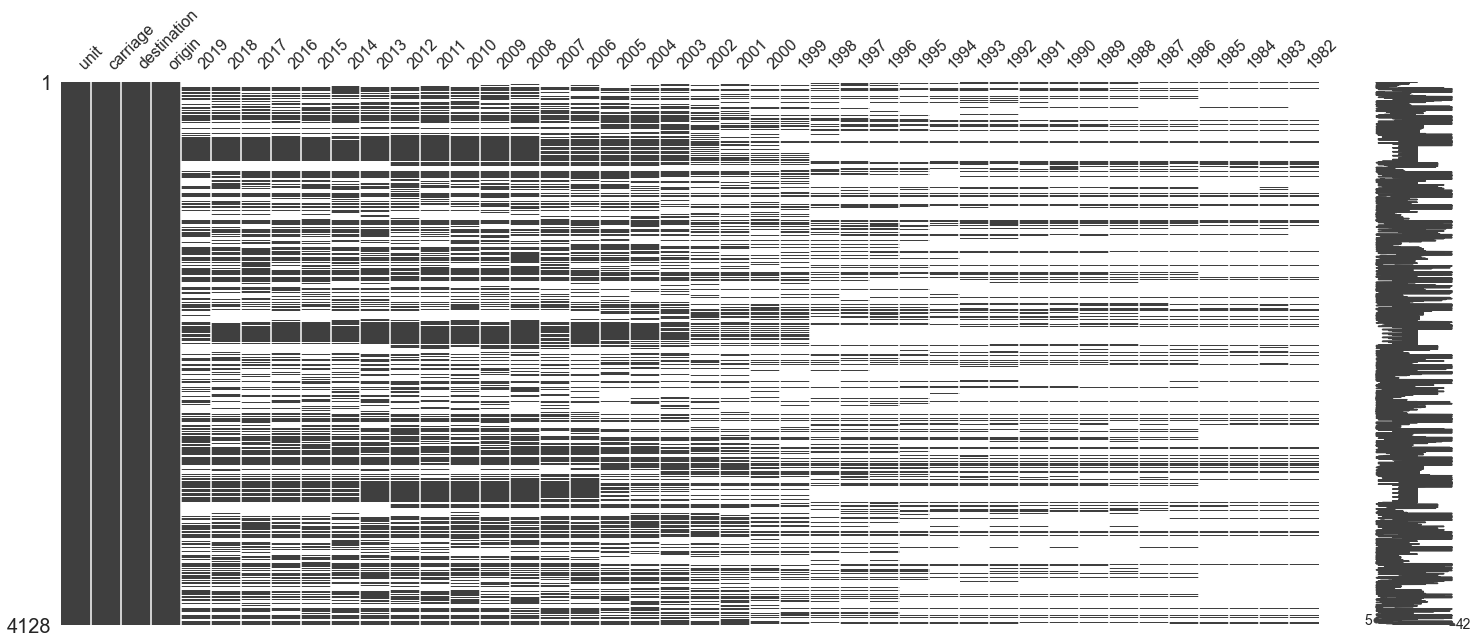
msno.matrix(df_load)

<AxesSubplot:>

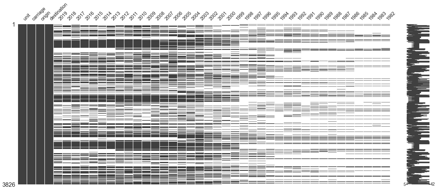
msno.matrix(df_unload)

<AxesSubplot:>

Here is brief look into the data

df_load.columns

Index(['unit', 'carriage', 'destination', 'origin', '2019', '2018', '2017',
       '2016', '2015', '2014', '2013', '2012', '2011', '2010', '2009', '2008',
       '2007', '2006', '2005', '2004', '2003', '2002', '2001', '2000', '1999',
       '1998', '1997', '1996', '1995', '1994', '1993', '1992', '1991', '1990',
       '1989', '1988', '1987', '1986', '1985', '1984', '1983', '1982'],
      dtype='object')

df_load.unit.unique()

array(['MIO_TKM'], dtype=object)

df_load.carriage.unique()

array(['HIRE', 'NOT_SPEC', 'OWN', 'TOT'], dtype=object)

• HIRE: hire or reward

• OWN:

df_load.destination.unique()

array(['AD', 'AF', 'AFR_N', 'AL', 'AM', 'AT', 'AZ', 'BA', 'BE', 'BG',
       'BH', 'BY', 'CH', 'CY', 'CZ', 'CZ_SK', 'DE', 'DK', 'DZ', 'EA',
       'EE', 'EEA_X_LI', 'EG', 'EH', 'EL', 'ES', 'EU15', 'EU25',
       'EU27_2007', 'EU27_2020', 'EU28', 'EUR_OTH', 'EXT_EU15', 'EX_DD',
       'EX_SU', 'EX_YU', 'FI', 'FR', 'GE', 'GI', 'HR', 'HU', 'IE', 'IL',
       'IQ', 'IR', 'IS', 'IT', 'JO', 'KG', 'KZ', 'LB', 'LI', 'LT', 'LU',
       'LV', 'MA', 'MC', 'MD', 'ME', 'MK', 'MN', 'MT', 'NE', 'NL', 'NO',
       'OTH', 'PL', 'PT', 'RO', 'RS', 'RS_ME', 'RU', 'SE', 'SI', 'SK',
       'SL', 'SM', 'SY', 'TJ', 'TM', 'TN', 'TR', 'UA', 'UK', 'UNK', 'US',
       'UZ', 'VA', 'WORLD', 'XK'], dtype=object)

df_load.origin.unique()

array(['CZ', 'DE', 'ES', 'FR', 'HU', 'LU', 'NL', 'PT', 'UK', 'LV', 'DK',
       'EL', 'EU15', 'IE', 'IT', 'AT', 'BE', 'BG', 'CY', 'FI', 'HR', 'RO',
       'SE', 'SI', 'LT', 'PL', 'SK', 'CH', 'EE', 'LI', 'NO'], dtype=object)

For the purpose of demonstration, we will only use part of the data.

• We will only look at 2019

• We will only look at HIRE

lunl_c_origin = [
    i for i in set.intersection(
        set(df_load.origin.unique()), 
        set(df_load.destination.unique())
    ) if len(i) == 2
]

df_load_selected = df_load[['unit', 'carriage', 'destination', 'origin', '2019', '2018', '2017', '2016', '2015', '2014', '2013', '2012', '2011', '2010']]
df_load_selected_com = df_load_selected.loc[
    (
        df_load_selected.carriage == "HIRE"
    ) & (
        df_load_selected.destination.isin(lunl_c_origin)
    ) & (
        df_load_selected.origin.isin(lunl_c_origin)
    ) 
]
df_load_selected_com#.sample(10)

	unit	carriage	destination	origin	2019	2018	2017	2016	2015	2014	2013	2012	2011	2010
48	MIO_TKM	HIRE	AT	BE	53.0	85.0	53.0	55.0	102.0	11.0	19.0	21.0	19.0	18.0
49	MIO_TKM	HIRE	AT	BG	126.0	97.0	229.0	119.0	147.0	95.0	220.0	131.0	66.0	46.0
50	MIO_TKM	HIRE	AT	CH	9.0	20.0	20.0	16.0	30.0	46.0	53.0	37.0	64.0	47.0
51	MIO_TKM	HIRE	AT	CY	0.0	0.0	1.0	1.0	0.0	0.0	0.0	1.0	0.0	1.0
52	MIO_TKM	HIRE	AT	CZ	454.0	478.0	678.0	577.0	700.0	779.0	722.0	651.0	572.0	589.0
...	...	...	...	...	...	...	...	...	...	...	...	...	...	...
1468	MIO_TKM	HIRE	UK	PT	460.0	380.0	617.0	742.0	516.0	270.0	403.0	366.0	408.0	236.0
1469	MIO_TKM	HIRE	UK	RO	211.0	371.0	314.0	390.0	420.0	370.0	281.0	280.0	364.0	514.0
1470	MIO_TKM	HIRE	UK	SE	NaN	NaN	3.0	NaN	NaN	NaN	4.0	5.0	12.0	1.0
1471	MIO_TKM	HIRE	UK	SI	121.0	176.0	135.0	193.0	211.0	157.0	221.0	144.0	197.0	186.0
1472	MIO_TKM	HIRE	UK	SK	353.0	421.0	293.0	441.0	278.0	233.0	421.0	234.0	476.0	208.0

788 rows × 14 columns

years = ['2019', '2018', '2017', '2016', '2015', '2014', '2013', '2012', '2011', '2010']

df_unload_19 = df_unload[['unit', 'carriage', 'origin', 'destination'] + years]
df_unload_19_com = df_unload_19.loc[
    (
        df_unload_19.carriage == "HIRE"
    ) & (
        df_unload_19.origin.apply(lambda x: len(x)==2)
    )  
]
df_unload_19_com.sample(10)

	unit	carriage	origin	destination	2019	2018	2017	2016	2015	2014	2013	2012	2011	2010
83	MIO_TKM	HIRE	BA	UK	NaN	NaN	NaN	NaN	NaN	NaN	NaN	NaN	NaN	NaN
1124	MIO_TKM	HIRE	RO	FR	NaN	NaN	NaN	NaN	NaN	7.0	NaN	NaN	NaN	NaN
54	MIO_TKM	HIRE	AT	NO	NaN	NaN	1.0	NaN	NaN	NaN	NaN	NaN	NaN	1.0
788	MIO_TKM	HIRE	IE	SI	NaN	NaN	NaN	NaN	NaN	NaN	NaN	NaN	NaN	NaN
1343	MIO_TKM	HIRE	UA	SK	6.0	6.0	5.0	10.0	91.0	28.0	44.0	17.0	39.0	8.0
1286	MIO_TKM	HIRE	SL	EL	NaN	NaN	NaN	NaN	NaN	NaN	NaN	NaN	NaN	NaN
898	MIO_TKM	HIRE	LU	LU	NaN	NaN	NaN	NaN	NaN	NaN	NaN	NaN	NaN	NaN
796	MIO_TKM	HIRE	IR	NL	NaN	NaN	NaN	NaN	NaN	NaN	NaN	NaN	NaN	NaN
707	MIO_TKM	HIRE	GE	PL	NaN	NaN	NaN	51.0	NaN	NaN	NaN	NaN	NaN	NaN
398	MIO_TKM	HIRE	ES	DE	378.0	344.0	464.0	303.0	538.0	535.0	586.0	814.0	950.0	1288.0

df_load_selected.to_csv("assets/road-freight-eurostats/eurostats_load_selected.csv")

11. Construct the Matrix

df_lunl = df_load_selected_com.pivot(index='origin', columns='destination', values='2019')
df_lunl

destination	AT	BE	BG	CH	CY	CZ	DE	DK	EE	EL	...	LV	NL	NO	PL	PT	RO	SE	SI	SK	UK
origin
AT	NaN	55.0	21.0	98.0	NaN	42.0	1404.0	18.0	NaN	31.0	...	NaN	62.0	17.0	10.0	NaN	NaN	45.0	27.0	33.0	36.0
BE	53.0	NaN	15.0	77.0	NaN	11.0	1102.0	23.0	NaN	NaN	...	NaN	807.0	NaN	36.0	31.0	NaN	NaN	5.0	NaN	152.0
BG	126.0	24.0	NaN	NaN	NaN	44.0	382.0	22.0	NaN	461.0	...	NaN	77.0	NaN	144.0	36.0	297.0	107.0	18.0	28.0	45.0
CH	9.0	22.0	NaN	NaN	NaN	NaN	191.0	NaN	NaN	NaN	...	NaN	13.0	NaN	NaN	NaN	NaN	NaN	NaN	NaN	20.0
CY	0.0	0.0	0.0	0.0	NaN	0.0	1.0	2.0	NaN	1.0	...	0.0	1.0	NaN	0.0	0.0	0.0	1.0	NaN	0.0	9.0
CZ	454.0	227.0	24.0	84.0	NaN	NaN	2317.0	58.0	NaN	37.0	...	NaN	304.0	45.0	201.0	26.0	17.0	73.0	33.0	631.0	137.0
DE	2050.0	1981.0	8.0	1752.0	NaN	443.0	NaN	1257.0	NaN	13.0	...	NaN	2741.0	106.0	432.0	306.0	32.0	270.0	25.0	59.0	689.0
DK	47.0	2.0	NaN	3.0	NaN	NaN	344.0	NaN	NaN	NaN	...	NaN	79.0	400.0	45.0	NaN	NaN	643.0	NaN	NaN	65.0
EE	11.0	NaN	NaN	NaN	NaN	NaN	194.0	22.0	NaN	NaN	...	108.0	54.0	15.0	41.0	NaN	NaN	88.0	NaN	NaN	NaN
EL	282.0	150.0	95.0	12.0	NaN	155.0	2358.0	95.0	NaN	NaN	...	NaN	533.0	NaN	156.0	83.0	141.0	72.0	NaN	39.0	289.0
ES	459.0	1511.0	39.0	768.0	NaN	226.0	8339.0	543.0	NaN	27.0	...	NaN	3586.0	166.0	451.0	3140.0	13.0	366.0	NaN	45.0	4054.0
FI	NaN	NaN	NaN	NaN	NaN	NaN	5.0	NaN	NaN	NaN	...	17.0	NaN	120.0	NaN	NaN	NaN	692.0	NaN	NaN	NaN
FR	28.0	1203.0	NaN	355.0	NaN	5.0	701.0	6.0	NaN	NaN	...	NaN	254.0	NaN	51.0	1.0	NaN	NaN	NaN	NaN	266.0
HR	172.0	96.0	1.0	24.0	NaN	51.0	432.0	22.0	NaN	NaN	...	NaN	68.0	NaN	30.0	NaN	21.0	13.0	184.0	21.0	58.0
HU	694.0	225.0	33.0	103.0	NaN	345.0	2203.0	75.0	12.0	38.0	...	11.0	279.0	23.0	149.0	39.0	231.0	30.0	141.0	243.0	273.0
IE	NaN	11.0	NaN	12.0	NaN	NaN	44.0	NaN	NaN	NaN	...	NaN	67.0	NaN	NaN	13.0	10.0	15.0	NaN	NaN	512.0
IT	294.0	292.0	NaN	659.0	NaN	7.0	1999.0	NaN	NaN	31.0	...	NaN	387.0	NaN	28.0	67.0	8.0	133.0	35.0	10.0	308.0
LI	NaN	NaN	NaN	NaN	NaN	NaN	NaN	NaN	NaN	NaN	...	NaN	NaN	NaN	NaN	NaN	NaN	NaN	NaN	NaN	NaN
LT	105.0	88.0	7.0	43.0	NaN	148.0	982.0	145.0	167.0	21.0	...	375.0	272.0	125.0	252.0	46.0	30.0	177.0	38.0	28.0	307.0
LU	5.0	105.0	NaN	5.0	NaN	NaN	148.0	1.0	NaN	NaN	...	NaN	58.0	0.0	2.0	NaN	NaN	NaN	NaN	NaN	3.0
LV	43.0	169.0	NaN	13.0	NaN	59.0	652.0	7.0	317.0	2.0	...	NaN	212.0	86.0	36.0	NaN	20.0	90.0	63.0	NaN	5.0
NL	99.0	3092.0	NaN	329.0	NaN	43.0	5428.0	393.0	15.0	50.0	...	NaN	NaN	194.0	41.0	13.0	15.0	723.0	8.0	7.0	769.0
NO	NaN	15.0	NaN	1.0	NaN	NaN	67.0	69.0	NaN	NaN	...	NaN	37.0	NaN	NaN	NaN	NaN	702.0	NaN	NaN	NaN
PL	1203.0	2799.0	151.0	270.0	NaN	2879.0	22471.0	1566.0	191.0	406.0	...	274.0	3701.0	203.0	NaN	219.0	1617.0	1779.0	668.0	1731.0	4602.0
PT	59.0	212.0	NaN	162.0	NaN	91.0	854.0	26.0	NaN	NaN	...	NaN	202.0	7.0	61.0	NaN	NaN	60.0	15.0	30.0	460.0
RO	404.0	654.0	64.0	66.0	NaN	249.0	2152.0	93.0	NaN	150.0	...	NaN	424.0	10.0	325.0	18.0	NaN	156.0	43.0	126.0	211.0
SE	NaN	14.0	NaN	2.0	NaN	NaN	181.0	36.0	1.0	16.0	...	NaN	37.0	646.0	1.0	NaN	NaN	NaN	NaN	NaN	NaN
SI	477.0	178.0	NaN	48.0	NaN	104.0	1248.0	55.0	NaN	63.0	...	13.0	214.0	36.0	121.0	16.0	25.0	53.0	NaN	65.0	121.0
SK	701.0	252.0	17.0	170.0	NaN	982.0	2263.0	62.0	NaN	NaN	...	0.0	247.0	6.0	167.0	NaN	163.0	57.0	81.0	NaN	353.0
UK	14.0	271.0	NaN	32.0	NaN	8.0	274.0	8.0	NaN	NaN	...	NaN	226.0	3.0	12.0	9.0	NaN	15.0	NaN	13.0	NaN

30 rows × 30 columns

fig, ax = plt.subplots(figsize=(30, 30))

sns.heatmap(
    df_lunl, annot=True, fmt="0.1f", linewidths=.5, ax=ax
)

<AxesSubplot:xlabel='destination', ylabel='origin'>

df_load_selected_com.head()

	unit	carriage	destination	origin	2019	2018	2017	2016	2015	2014	2013	2012	2011	2010
48	MIO_TKM	HIRE	AT	BE	53.0	85.0	53.0	55.0	102.0	11.0	19.0	21.0	19.0	18.0
49	MIO_TKM	HIRE	AT	BG	126.0	97.0	229.0	119.0	147.0	95.0	220.0	131.0	66.0	46.0
50	MIO_TKM	HIRE	AT	CH	9.0	20.0	20.0	16.0	30.0	46.0	53.0	37.0	64.0	47.0
51	MIO_TKM	HIRE	AT	CY	0.0	0.0	1.0	1.0	0.0	0.0	0.0	1.0	0.0	1.0
52	MIO_TKM	HIRE	AT	CZ	454.0	478.0	678.0	577.0	700.0	779.0	722.0	651.0	572.0	589.0

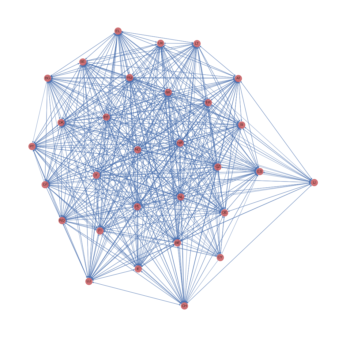
D = nx.from_pandas_edgelist(df_load_selected_com, "origin", "destination", edge_attr="2019", create_using=nx.DiGraph)

fig, ax = plt.subplots(figsize=(20, 20))
nx_draw_options = {
    "node_color": "r",
    "node_size": 500, 
    "alpha": 0.8,
    "edge_color": "b"
}
nx.draw(D, pos=nx.spring_layout(D, k=0.9, iterations=50), ax=ax, with_labels=True, **nx_draw_options)

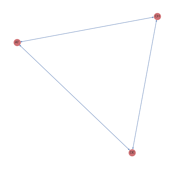
11.1. Build a Minimal Network

lunl_minimal = ["AT", "CH", "DE"]
df_lunl_minimal = {}
for year in years:
    df_lunl_minimal[year] = df_load_selected_com.pivot(index='origin', columns='destination', values=year).loc[lunl_minimal, lunl_minimal]
    
df_lunl_minimal;

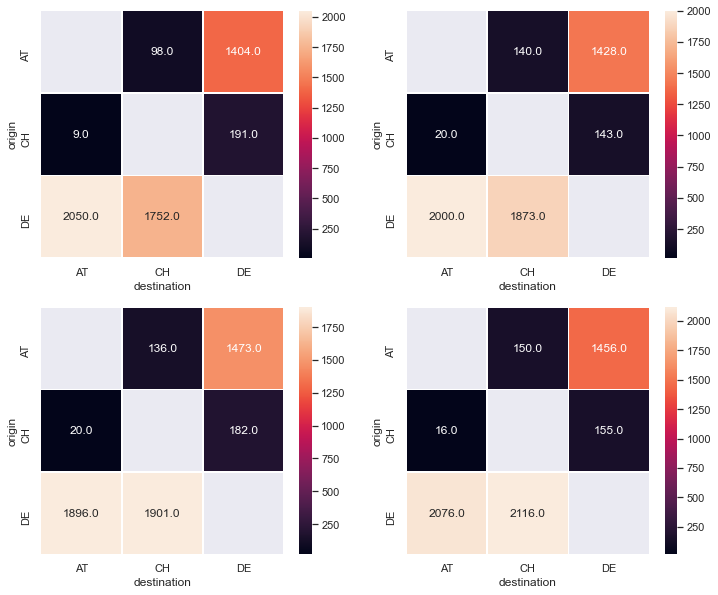
fig, ax = plt.subplots(nrows=2, ncols=2, figsize=(12, 10))

sns.heatmap(
    df_lunl_minimal["2019"], annot=True, fmt="0.1f", linewidths=.5, ax=ax[0,0]
)

sns.heatmap(
    df_lunl_minimal["2018"], annot=True, fmt="0.1f", linewidths=.5, ax=ax[0,1]
)

sns.heatmap(
    df_lunl_minimal["2017"], annot=True, fmt="0.1f", linewidths=.5, ax=ax[1,0]
)

sns.heatmap(
    df_lunl_minimal["2016"], annot=True, fmt="0.1f", linewidths=.5, ax=ax[1,1]
)

<AxesSubplot:xlabel='destination', ylabel='origin'>

D_minimal = nx.DiGraph(df_lunl_minimal["2019"])

fig, ax = plt.subplots(figsize=(10, 10))
nx_draw_options = {
    "node_color": "r",
    "node_size": 500, 
    "alpha": 0.8,
    "edge_color": "b"
}
nx.draw(D_minimal, pos=nx.spring_layout(D, k=0.4, iterations=10), ax=ax, with_labels=True, **nx_draw_options)

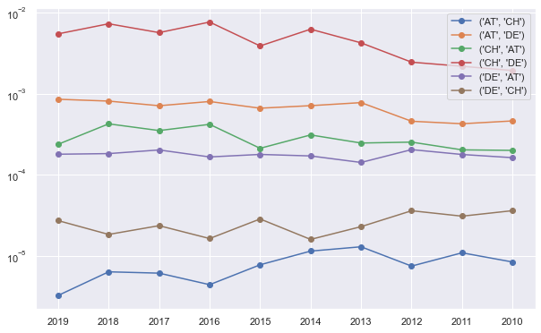
12. Naive Model

A naive idea is that the demand on the lane depends on the total demand of the origin and the total demand of the destination.

def naive_model_kpq(o_t, d_t, data):
    
    k_pq = {}
    for p in o_t:
        for q in d_t:
            if p != q:
                k_pq[(p,q)] = data[p][q] / (o_t[p] * d_t[q])
        
    return k_pq

def naive_model(p, q, k_pq, o_t, d_t):
    
    g_pq = k_pq[(p,q)] * (o_t[p] * d_t[q])
        
    return g_pq

df_lunl_minimal["2019"].to_dict()

{'AT': {'AT': nan, 'CH': 9.0, 'DE': 2050.0},
 'CH': {'AT': 98.0, 'CH': nan, 'DE': 1752.0},
 'DE': {'AT': 1404.0, 'CH': 191.0, 'DE': nan}}

total_demand_origin["2019"]

{'AT': 1502.0, 'CH': 200.0, 'DE': 3802.0}

total_demand_dest["2019"]

{'AT': 2059.0, 'CH': 1850.0, 'DE': 1595.0}

naive_kpqs = {}
for year in years:
    naive_kpqs[year] = naive_model_kpq(total_demand_origin[year], total_demand_dest[year], df_lunl_minimal[year].to_dict())

naive_kpqs[year]

{('AT', 'CH'): 8.37794141501648e-06,
 ('AT', 'DE'): 0.00046207319268525015,
 ('CH', 'AT'): 0.00020008003201280514,
 ('CH', 'DE'): 0.0019352568613652356,
 ('DE', 'AT'): 0.00016255303019258526,
 ('DE', 'CH'): 3.604375661642385e-05}

fig, ax = plt.subplots(figsize=(10, 6.18))

for key in naive_kpqs[year]:
    ax.plot(
        naive_kpqs.keys(),
        [val[key] for idx, val in naive_kpqs.items()],
        "-",
        marker="o",
        label=key
    )
    
ax.set_yscale("log")
plt.legend()

<matplotlib.legend.Legend at 0x7fadfa5c7e90>

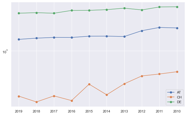
total_demand_origin

{'2019': {'AT': 1502.0, 'CH': 200.0, 'DE': 3802.0},
 '2018': {'AT': 1568.0, 'CH': 163.0, 'DE': 3873.0},
 '2017': {'AT': 1609.0, 'CH': 202.0, 'DE': 3797.0},
 '2016': {'AT': 1606.0, 'CH': 171.0, 'DE': 4192.0},
 '2015': {'AT': 1681.0, 'CH': 306.0, 'DE': 4205.0},
 '2014': {'AT': 1685.0, 'CH': 210.0, 'DE': 4310.0},
 '2013': {'AT': 1661.0, 'CH': 310.0, 'DE': 4545.0},
 '2012': {'AT': 2042.0, 'CH': 410.0, 'DE': 4268.0},
 '2011': {'AT': 2292.0, 'CH': 439.0, 'DE': 4740.0},
 '2010': {'AT': 2253.0, 'CH': 476.0, 'DE': 4780.0}}

fig, ax = plt.subplots(figsize=(10, 6.18))

for key in total_demand_origin["2019"]:
    ax.plot(
        total_demand_origin.keys(),
        [val[key] for idx, val in total_demand_origin.items()],
        "-",
        marker="o",
        label=key
    )
    
ax.set_yscale("log")
plt.legend()

<matplotlib.legend.Legend at 0x7fadfa269810>

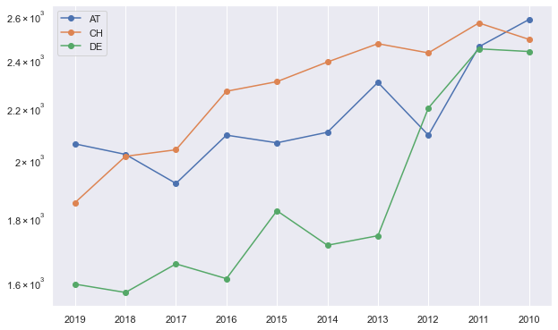
fig, ax = plt.subplots(figsize=(10, 6.18))

for key in total_demand_dest["2019"]:
    ax.plot(
        total_demand_origin.keys(),
        [val[key] for idx, val in total_demand_dest.items()],
        "-",
        marker="o",
        label=key
    )
    
ax.set_yscale("log")
plt.legend()

<matplotlib.legend.Legend at 0x7fadfb5bce90>

validate_year = "2018"

naive_kpq = naive_kpqs["2017"]

for i_o in lunl_minimal:
    for i_d in lunl_minimal:
        if i_o != i_d:
            print(
                f"({i_o}, {i_d}):",
                naive_model(i_o, i_d, naive_kpq, total_demand_origin[validate_year], total_demand_dest[validate_year])
            )

(AT, CH): 19.260730555573353
(AT, DE): 1753.906890057625
(CH, AT): 115.69937369519833
(CH, DE): 1456.1178935718347
(DE, AT): 1584.0376921017196
(DE, CH): 183.45562557526424

df_lunl_minimal[validate_year].to_dict()

{'AT': {'AT': nan, 'CH': 20.0, 'DE': 2000.0},
 'CH': {'AT': 140.0, 'CH': nan, 'DE': 1873.0},
 'DE': {'AT': 1428.0, 'CH': 143.0, 'DE': nan}}

df_lunl_minimal["2017"].to_dict()

{'AT': {'AT': nan, 'CH': 20.0, 'DE': 1896.0},
 'CH': {'AT': 136.0, 'CH': nan, 'DE': 1901.0},
 'DE': {'AT': 1473.0, 'CH': 182.0, 'DE': nan}}

df_lunl_minimal["2018"] - df_lunl_minimal["2017"]

destination	AT	CH	DE
origin
AT	NaN	4.0	-45.0
CH	0.0	NaN	-39.0
DE	104.0	-28.0	NaN

total_demand_origin["2015"]

{'AT': 1681.0, 'CH': 306.0, 'DE': 4205.0}

total_demand_dest["2015"]

{'AT': 2063.0, 'CH': 2306.0, 'DE': 1823.0}

mass_multiplications = {}
for year in years:
    df_mass_mul_year = pd.DataFrame(
        np.outer(
            list(total_demand_origin[year].values()),
            list(total_demand_dest[year].values())
        ),
        columns=total_demand_origin[year].keys()
    )

    df_mass_mul_year.index = total_demand_origin[year].keys()
    mass_multiplications[year] = df_mass_mul_year.copy()

mass_multiplications["2018"]

	AT	CH	DE
AT	3167360.0	3156384.0	2463328.0
CH	329260.0	328119.0	256073.0
DE	7823460.0	7796349.0	6084483.0

year_1 = "2014"
year_2 = "2015"

df_mass_mul_diff = mass_multiplications[year_2] - mass_multiplications[year_1]
df_mass_mul_diff[df_mass_mul_diff >0] = 1
df_mass_mul_diff[df_mass_mul_diff <0] = -1
df_mass_mul_diff.values[[np.arange(df_mass_mul_diff.shape[0])]*2] = np.nan



df_demand_diff = df_lunl_minimal[year_2] - df_lunl_minimal[year_1]
df_demand_diff[df_demand_diff >0] = 1
df_demand_diff[df_demand_diff <0] = -1

fig, ax = plt.subplots(ncols=2, figsize=(10,5))

ax[0].matshow(df_mass_mul_diff)
ax[1].matshow(df_demand_diff)

/Users/leima/anaconda3/envs/theflow-code/lib/python3.7/site-packages/ipykernel_launcher.py:7: FutureWarning: Using a non-tuple sequence for multidimensional indexing is deprecated; use `arr[tuple(seq)]` instead of `arr[seq]`. In the future this will be interpreted as an array index, `arr[np.array(seq)]`, which will result either in an error or a different result.
  import sys

<matplotlib.image.AxesImage at 0x7fadfb8cf850>

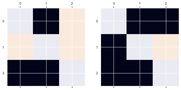
df_demand_diff

destination	AT	CH	DE
origin
AT	NaN	-1.0	-1.0
CH	-1.0	NaN	1.0
DE	-1.0	-1.0	NaN

13. Four Stage Model

df_load_selected_com_minimal = df_load_selected_com.loc[
    (
        df_load_selected_com.origin.isin(lunl_minimal)
    ) & (
        df_load_selected_com.destination.isin(lunl_minimal)
    )
]
df_load_selected_com_minimal

	unit	carriage	destination	origin	2019	2018	2017	2016	2015	2014	2013	2012	2011	2010
50	MIO_TKM	HIRE	AT	CH	9.0	20.0	20.0	16.0	30.0	46.0	53.0	37.0	64.0	47.0
53	MIO_TKM	HIRE	AT	DE	2050.0	2000.0	1896.0	2076.0	2033.0	2057.0	2250.0	2055.0	2393.0	2536.0
186	MIO_TKM	HIRE	CH	AT	98.0	140.0	136.0	150.0	134.0	137.0	176.0	217.0	219.0	246.0
191	MIO_TKM	HIRE	CH	DE	1752.0	1873.0	1901.0	2116.0	2172.0	2253.0	2295.0	2213.0	2347.0	2244.0
261	MIO_TKM	HIRE	DE	AT	1404.0	1428.0	1473.0	1456.0	1547.0	1548.0	1485.0	1825.0	2073.0	2007.0
264	MIO_TKM	HIRE	DE	CH	191.0	143.0	182.0	155.0	276.0	164.0	257.0	373.0	375.0	429.0
267	MIO_TKM	HIRE	DE	DE	NaN	NaN	NaN	NaN	NaN	NaN	NaN	NaN	NaN	NaN

df_load_selected_com_minimal_origin = df_load_selected_com_minimal.groupby("origin").sum()
df_load_selected_com_minimal_origin

	2019	2018	2017	2016	2015	2014	2013	2012	2011	2010
origin
AT	1502.0	1568.0	1609.0	1606.0	1681.0	1685.0	1661.0	2042.0	2292.0	2253.0
CH	200.0	163.0	202.0	171.0	306.0	210.0	310.0	410.0	439.0	476.0
DE	3802.0	3873.0	3797.0	4192.0	4205.0	4310.0	4545.0	4268.0	4740.0	4780.0

df_load_selected_com_minimal_dest = df_load_selected_com_minimal.groupby("destination").sum()
df_load_selected_com_minimal_dest

	2019	2018	2017	2016	2015	2014	2013	2012	2011	2010
destination
AT	2059.0	2020.0	1916.0	2092.0	2063.0	2103.0	2303.0	2092.0	2457.0	2583.0
CH	1850.0	2013.0	2037.0	2266.0	2306.0	2390.0	2471.0	2430.0	2566.0	2490.0
DE	1595.0	1571.0	1655.0	1611.0	1823.0	1712.0	1742.0	2198.0	2448.0	2436.0

total_demand_dest = df_load_selected_com_minimal_dest.to_dict()
total_demand_origin = df_load_selected_com_minimal_origin.to_dict()

14. Build a Symmetric Linear Model

from sympy.solvers import solve
from sympy import Symbol

lunl_minimal

['AT', 'CH', 'DE']

f12_s = Symbol("f12")
f13_s = Symbol("f13")
f23_s = Symbol("f23")

sols_s = {}
for year in years:
    d1, d2, d3 = [total_demand_dest[year][i] for i in lunl_minimal]

    eqns = [
        f12_s * d2 + f13_s * d3 - 1,
        f12_s * d1 + f23_s * d3 - 1,
        f13_s * d1 + f23_s * d2 - 1
    ]
    sols_s[year] = solve(eqns, f12_s, f13_s, f23_s, dict=True)[0]
    
print(sols_s)

{'2019': {f12: 0.000303742304713650, f13: 0.000274656260990437, f23: 0.000234855545200373}, '2018': {f12: 0.000302735191551942, f13: 0.000248627663530198, f23: 0.000247278747972678}, '2017': {f12: 0.000294397077859187, f13: 0.000241881058852468, f23: 0.000263404953970874}, '2016': {f12: 0.000289739080834145, f13: 0.000213191336331364, f23: 0.000244485315266896}, '2015': {f12: 0.000267589995791711, f13: 0.000210058952114270, f23: 0.000245727832518760}, '2014': {f12: 0.000276652003414130, f13: 0.000197898196168358, f23: 0.000244276189731357}, '2013': {f12: 0.000266398955631746, f13: 0.000196170023326037, f23: 0.000221861771056308}, '2012': {f12: 0.000228579971516024, f13: 0.000202252351781648, f23: 0.000237402502087569}, '2011': {f12: 0.000204213961033914, f13: 0.000194439124177686, f23: 0.000203531984370781}, '2010': {f12: 0.000205001189426696, f13: 0.000200963480430019, f23: 0.000193137080341069}}

Define the model

float(sols_s["2019"][f12_s])

0.00030374230471365

def gravity_model(coef_o_d, op, dq, all_coeff):
    
    g = float(all_coeff[coef_o_d] * op * dq)
    
    return g    

total_demand_origin["2019"]["AT"]

1502.0

gravity_model(f12_s, total_demand_origin["2019"]["AT"], total_demand_dest["2019"]["CH"], sols_s["2019"])

844.0087421078192

gravity_model(f13_s, total_demand_origin["2019"]["AT"], total_demand_dest["2019"]["DE"], sols_s["2019"])

657.9912578921808

gravity_model(f23_s, total_demand_origin["2019"]["CH"], total_demand_dest["2019"]["DE"], sols_s["2019"])

74.91891891891892

The results are far from being correct

15. Introduce Symmetry Breaking

lunl_minimal

['AT', 'CH', 'DE']

f12 = Symbol("f12")
f13 = Symbol("f13")
f21 = Symbol("f21")
f23 = Symbol("f23")
f31 = Symbol("f31")
f32 = Symbol("f32")

sols = {}
for year in years:

    d1, d2, d3 = [total_demand_dest[year][i] for i in lunl_minimal]

    eqns = [
        f12 * d2 + f13 * d3 - 1,
        f21 * d1 + f23 * d3 - 1,
        f31 * d1 + f32 * d2 - 1
    ]
    sols[year] = solve(eqns, f12, f13, f21, f23, f31, f32, dict=True)[0]
    
print(sols)

{'2019': {f31: 0.000485672656629432 - 0.898494414764449*f32, f21: 0.000485672656629432 - 0.774647887323944*f23, f12: 0.000540540540540541 - 0.862162162162162*f13}, '2018': {f31: 0.000495049504950495 - 0.996534653465347*f32, f21: 0.000495049504950495 - 0.777722772277228*f23, f12: 0.000496770988574267 - 0.780427223050174*f13}, '2017': {f31: 0.000521920668058455 - 1.06315240083507*f32, f21: 0.000521920668058455 - 0.863778705636743*f23, f12: 0.000490918016691213 - 0.812469317623957*f13}, '2016': {f31: 0.000478011472275335 - 1.08317399617591*f32, f21: 0.000478011472275335 - 0.770076481835564*f23, f12: 0.000441306266548985 - 0.710944395410415*f13}, '2015': {f31: 0.000484730974309258 - 1.11778962675715*f32, f21: 0.000484730974309258 - 0.883664566165778*f23, f12: 0.000433651344319167 - 0.790546400693842*f13}, '2014': {f31: 0.000475511174512601 - 1.13647170708512*f32, f21: 0.000475511174512601 - 0.814075130765573*f23, f12: 0.000418410041841004 - 0.716317991631799*f13}, '2013': {f31: 0.000434216239687364 - 1.07294832826748*f32, f21: 0.000434216239687364 - 0.756404689535389*f23, f12: 0.000404694455685957 - 0.704977741804937*f13}, '2012': {f31: 0.000478011472275335 - 1.16156787762906*f32, f21: 0.000478011472275335 - 1.05066921606119*f23, f12: 0.000411522633744856 - 0.904526748971193*f13}, '2011': {f31: 0.000407000407000407 - 1.04436304436304*f32, f21: 0.000407000407000407 - 0.996336996336996*f23, f12: 0.00038971161340608 - 0.954014029618083*f13}, '2010': {f31: 0.000387146728610143 - 0.963995354239257*f32, f21: 0.000387146728610143 - 0.943089430894309*f23, f12: 0.000401606425702811 - 0.978313253012048*f13}}

year_slice = 3

system_y = np.array([1, 1, 1] * len(years[:year_slice]))

system_A_nested = [[
        [total_demand_origin[year]["CH"], total_demand_origin[year]["DE"], 0, 0, 0, 0],
        [0, 0, total_demand_origin[year]["AT"], total_demand_origin[year]["DE"], 0, 0],
        [0, 0, 0, 0, total_demand_origin[year]["AT"], total_demand_origin[year]["CH"]]
    ] for year in years[:year_slice]
]

system_A = np.array(
    [item for sublist in system_A_nested for item in sublist]
)
system_A_T = np.transpose(system_A)

system_x = np.matmul(
    np.matmul(
        system_A_T,
        np.linalg.pinv(
            np.matmul(
                system_A, system_A_T,
            )
        )
    ),
    system_y
)

system_x

array([4.62077592e-04, 2.38748790e-04, 4.80157321e-05, 2.41902148e-04,
       5.76484352e-04, 5.31941301e-04])

system_x[0] * total_demand_origin["2019"]["AT"] * total_demand_dest["2019"]["CH"]

1283.9750053370456

system_x[1] * total_demand_origin["2019"]["AT"] * total_demand_dest["2019"]["DE"]

571.968089786805

fig, ax = plt.subplots(figsize=(12, 10))

sns.heatmap(
    df_lunl_minimal["2019"], annot=True, fmt="0.1f", linewidths=.5, ax=ax
)

<AxesSubplot:xlabel='destination', ylabel='origin'>

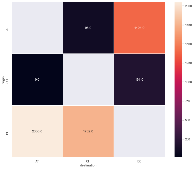
The results are still not as expected! We need to introduce more knowledge in to the coefficients. Now we need to introduce the gravity model!