7. Space Explorations

import pandas as pd

import datetime

import numpy as np

import matplotlib.pyplot as plt

import seaborn as sns
sns.set(style="darkgrid")

%%bash
ls data

air-transport-passengers-by-year.csv
air-transport-passengers-carried.csv
air-transportation-and-death-by-year.csv
space-exploration-launches-by-year.csv
space-exploration-world-and-china-launches-by-year.csv
space-exploration.csv

df_raw = pd.read_csv('data/space-exploration.csv')

df = df_raw.copy()

df.dtypes

Date                                  object
Event leading to space exploration    object
Country                               object
Researcher(s)                         object
dtype: object

df.iloc[21]

Date                                                                          6/20/1944
Event leading to space exploration    V-2 Rocket (MW 18014): First man-made object t...
Country                                                                         Germany
Researcher(s)                                                                 Wehrmacht
Name: 21, dtype: object

datetime.datetime.strptime('6/20/1944', '%m/%d/%Y')

datetime.datetime(1944, 6, 20, 0, 0)

def transform_date(inp):
    
    if '/' in str(inp):
        try:
            dt = datetime.datetime.strptime(inp, '%m/%d/%Y')
        except:
            dt = None
            pass
    else:
        dt = None
    
    return dt

df['dt_dates'] = df['Date'].apply( transform_date )
df['year'] = df['dt_dates'].apply( lambda x: x.year )
df['month'] = df['dt_dates'].apply( lambda x: x.month )
df['day'] = df['dt_dates'].apply( lambda x: x.day )

df_with_dates = df[~df.dt_dates.isna()]

df_with_dates['year'] = df_with_dates.year.astype(int)
df_with_dates['month'] = df_with_dates.month.astype(int)
df_with_dates['day'] = df_with_dates.day.astype(int)

/Users/leima/anaconda3/lib/python3.6/site-packages/ipykernel_launcher.py:1: SettingWithCopyWarning: 
A value is trying to be set on a copy of a slice from a DataFrame.
Try using .loc[row_indexer,col_indexer] = value instead

See the caveats in the documentation: http://pandas.pydata.org/pandas-docs/stable/indexing.html#indexing-view-versus-copy
  """Entry point for launching an IPython kernel.
/Users/leima/anaconda3/lib/python3.6/site-packages/ipykernel_launcher.py:2: SettingWithCopyWarning: 
A value is trying to be set on a copy of a slice from a DataFrame.
Try using .loc[row_indexer,col_indexer] = value instead

See the caveats in the documentation: http://pandas.pydata.org/pandas-docs/stable/indexing.html#indexing-view-versus-copy
  
/Users/leima/anaconda3/lib/python3.6/site-packages/ipykernel_launcher.py:3: SettingWithCopyWarning: 
A value is trying to be set on a copy of a slice from a DataFrame.
Try using .loc[row_indexer,col_indexer] = value instead

See the caveats in the documentation: http://pandas.pydata.org/pandas-docs/stable/indexing.html#indexing-view-versus-copy
  This is separate from the ipykernel package so we can avoid doing imports until

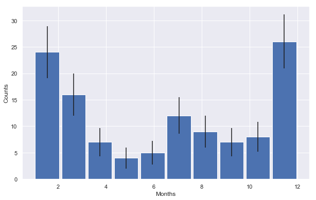
plt.figure( figsize=(10,6.18) )
import numpy as np
import pylab as plt

data       = df_with_dates.month.values
y,binEdges = np.histogram(data,bins=10)
bincenters = 0.5*(binEdges[1:]+binEdges[:-1])
menStd     = np.sqrt(y)
width      = 1
plt.bar(bincenters, y, width=width, yerr=menStd)
plt.xlabel('Months')
plt.ylabel('Counts')
plt.show()

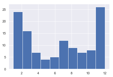
df_with_dates.month.hist()
plt.show()

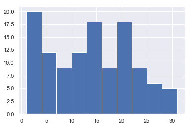
df_with_dates.day.hist()
plt.show()

7.1. Produce Pretty Graph

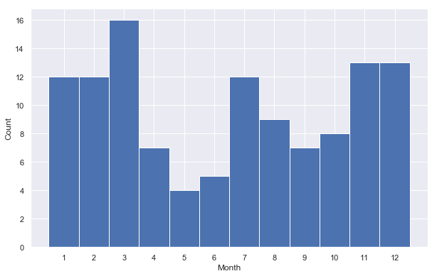
df_with_dates.groupby('month').count()[ 'dt_dates']

month
1     12
2     12
3     16
4      7
5      4
6      5
7     12
8      9
9      7
10     8
11    13
12    13
Name: dt_dates, dtype: int64

month_hist, month_edge = np.histogram(df_with_dates.month.values, bins = np.arange(1,14))
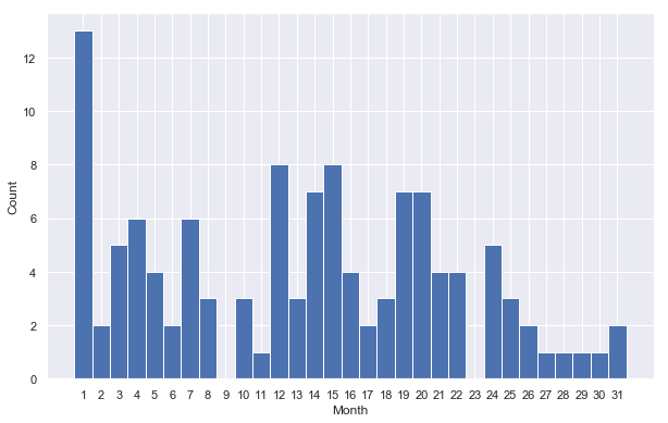
day_hist, day_edge = np.histogram(df_with_dates.day.values, bins = np.arange(1,33))

month_edge

array([ 1,  2,  3,  4,  5,  6,  7,  8,  9, 10, 11, 12, 13])

month_hist

array([12, 12, 16,  7,  4,  5, 12,  9,  7,  8, 13, 13])

fig, ax = plt.subplots( figsize=(10, 6.18) )

month_x = month_edge[:-1] -0.5
ax.bar( month_x, month_hist, 1, color=(0.2980392156862745, 0.4470588235294118, 0.6901960784313725) )

ax.set_xticks( np.arange(1,13) -0.5 )
ax.set_xticklabels( [ str(i) for i in np.arange(1,13) ] )

ax.set_xlabel('Month')
ax.set_ylabel('Count')

fig.savefig('export/month-distribution.png')

fig, ax = plt.subplots( figsize=(10, 6.18) )

day_x = day_edge[:-1] -0.5
ax.bar( day_x, day_hist, 1, color=(0.2980392156862745, 0.4470588235294118, 0.6901960784313725) )

ax.set_xticks( np.arange(1,32) -0.5 )
ax.set_xticklabels( [ str(i) for i in np.arange(1,32) ] )

ax.set_xlabel('Month')
ax.set_ylabel('Count')

fig.savefig('export/day-distribution.png')

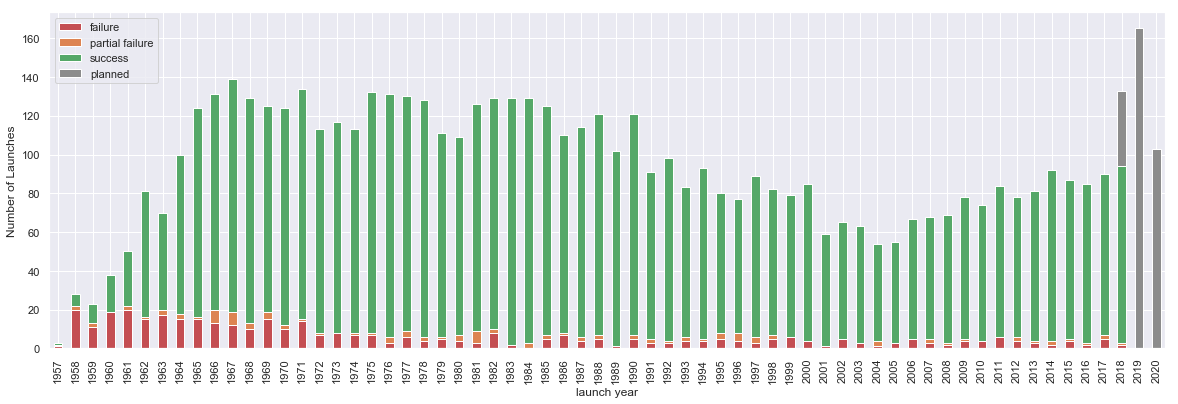
== Orbital launches by year ==

def comma_strings_to_int(inp):
    
    ret = inp.split(':')
    
    ret = [ int(i) for i in ret ]
    
    return ret

comma_strings_to_int('70: 78: 72: 77: 88: 82: 82:  83: 90:  0')

[70, 78, 72, 77, 88, 82, 82, 83, 90, 0]

launch_years = np.arange(1957, 2021,1) #[ 1957,1958,1959, 1960, ... ]
failures = [ [1, 20, 11], [19, 20, 15, 17, 15, 15, 13, 12, 10, 15] , [10, 14, 7, 8, 7, 7, 3, 6, 4, 5], [4, 3, 8, 2, 0, 5, 7, 4, 5, 1], [5, 3, 3, 4, 4, 5, 4, 3, 5, 6], [4, 1, 5, 3, 1, 3, 5, 3, 2, 4], [4, 6, 4, 3, 2, 4, 2, 5, 2, 0], [0]  ]
partial_failures = [ [1, 2, 2], [0, 2, 1, 3, 3, 1, 7, 7, 3, 4], [2, 1, 1, 0, 1, 1, 3, 3, 2, 1], [3, 6, 2, 0, 3, 2, 1, 2, 2, 0], [2, 2, 1, 2, 1, 3, 4, 3, 2, 0], [0, 0, 0, 0, 3, 0, 0, 2, 1, 1], [0, 0, 2, 1, 2, 1, 1, 2, 1, 0], [0] ]
success = [ [1, 6, 10], [19, 28, 65, 50, 82, 108, 111, 120, 116, 106],  [112, 119, 105, 109, 105, 124, 125, 121, 122, 105], [102, 117, 119, 127, 126, 118, 102, 108, 114, 101], [114, 86, 94, 77, 88, 72, 69, 83, 75, 73], [81, 58, 60, 60, 50, 52, 62, 63, 66, 73], [70, 78, 72, 77, 88, 82, 82, 83, 91, 0], [0] ]
planned = [[0, 0, 0], [0, 0, 0, 0, 0, 0, 0, 0, 0, 0], [0, 0, 0, 0, 0, 0, 0, 0, 0, 0], [0, 0, 0, 0, 0, 0, 0, 0, 0, 0], [0, 0, 0, 0, 0, 0, 0, 0, 0, 0], [0, 0, 0, 0, 0, 0, 0, 0, 0, 0], [0, 0, 0, 0, 0, 0, 0, 0, 39, 165], [103] ]

df_launches = pd.DataFrame( { 
    'launch year': launch_years, 
    'failure': [item for sublist in failures for item in sublist], 
    'partial failure': [item for sublist in partial_failures for item in sublist], 
    'success': [item for sublist in success for item in sublist], 
    'planned': [item for sublist in planned for item in sublist] } )
df_launches.set_index('launch year', inplace=True);

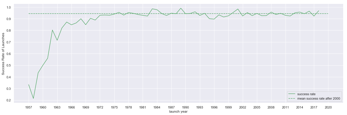
df_launches['success rate'] = df_launches.apply( lambda x: x['success'] / (x['failure'] + x['partial failure'] + x['success']) , axis=1)

/Users/leima/anaconda3/lib/python3.6/site-packages/ipykernel_launcher.py:1: RuntimeWarning: invalid value encountered in long_scalars
  """Entry point for launching an IPython kernel.

df_launches['mean success rate after 2000'] = df_launches[ ['success rate' ] ].loc[2000:].describe().loc['mean'].values[0]
df_launches['std success rate after 2000'] = df_launches[ ['success rate' ] ].loc[2000:].describe().loc['std'].values[0]

df_launches.head()

	failure	partial failure	success	planned	success rate	mean success rate after 2000	std success rate after 2000
launch year
1957	1	1	1	0	0.333333	0.943651	0.017766
1958	20	2	6	0	0.214286	0.943651	0.017766
1959	11	2	10	0	0.434783	0.943651	0.017766
1960	19	0	19	0	0.500000	0.943651	0.017766
1961	20	2	28	0	0.560000	0.943651	0.017766

df_launches.to_csv('data/space-exploration-launches-by-year.csv')

current_palette = sns.color_palette()
print(current_palette)
sns.palplot(current_palette)

[(0.2980392156862745, 0.4470588235294118, 0.6901960784313725), (0.8666666666666667, 0.5176470588235295, 0.3215686274509804), (0.3333333333333333, 0.6588235294117647, 0.40784313725490196), (0.7686274509803922, 0.3058823529411765, 0.3215686274509804), (0.5058823529411764, 0.4470588235294118, 0.7019607843137254), (0.5764705882352941, 0.47058823529411764, 0.3764705882352941), (0.8549019607843137, 0.5450980392156862, 0.7647058823529411), (0.5490196078431373, 0.5490196078431373, 0.5490196078431373), (0.8, 0.7254901960784313, 0.4549019607843137), (0.39215686274509803, 0.7098039215686275, 0.803921568627451)]

fig, ax = plt.subplots( figsize=(20,6.18) )

df_launches[ ['failure', 'partial failure', 'success', 'planned' ] ].plot.bar(stacked=True, ax=ax, color= ['r',(0.8666666666666667, 0.5176470588235295, 0.3215686274509804), (0.3333333333333333, 0.6588235294117647, 0.40784313725490196), (0.5490196078431373, 0.5490196078431373, 0.5490196078431373)] )
ax.set_xticklabels( launch_years );
ax.set_ylabel('Number of Launches')
fig.savefig('export/space-launch-yearly.png')

fig, ax = plt.subplots( figsize=(20,6.18) )

df_launches[ ['success rate', 'mean success rate after 2000' ] ].plot(ax=ax, color= 'g', style=['-', '--'] )
ax.set_xticks( launch_years[::3] )
ax.set_xticklabels( launch_years[::3] );
ax.set_ylabel('Success Rate of Launches')
fig.savefig('export/space-launch-success-rate-yearly.png')

7.2. Chinese Rocket Launches

== Launch statistics ==

<!-- The summary and bar chart are constantly getting out of sync.  Make sure to update both of them at the same time. -->

Rockets from the Long March family have accumulated 290 launches {{as of|2018|11|01|lc=on}}. Of these, 275 were successful, 8 were failures, and 7 were partial failures. The cumulative success rate is {{percent|275|290|1}}.

<!-- Bars are grouped in decades, with extra spaces between the groups.  -->

{{ #invoke:Chart | bar-chart
| height = 400
| width = 900
| stack = 1
| group 1 =   0:  0:  0:  0:  1:  0:  0:  0:  0:  0:      0:  0:  0:  0:  0:  0:  0:  0:  0:  0:      0:  0:  1:  0:  0:  1:  1:  0:  0:  0:      0:  0:  0:  0:  0:  0:  0:  0:  0:  0:      0:  1:  0:  1:  0:  0:  1:  1:  0:  0:      0
| group 2 =   0:  0:  0:  0:  0:  0:  0:  0:  0:  0:      0:  0:  0:  0:  1:  0:  0:  0:  0:  0:      0:  1:  0:  0:  0:  0:  1:  0:  0:  0:      0:  0:  0:  0:  0:  0:  0:  0:  0:  1:      0:  0:  0:  0:  0:  0:  1:  1:  0:  0:      0
| group 3 =   1:  1:  0:  0:  0:  1:  1:  0:  1:  0:      0:  0:  1:  1:  2:  1:  2:  2:  4:  0:      5:  0:  3:  1:  5:  1:  2:  6:  6:  4:      5:  1:  4:  6:  8:  5:  6: 10: 11:  5:     15: 18: 19: 13: 15: 19: 20: 15: 30:  0:      0
| group 4 =   0:  0:  0:  0:  0:  0:  0:  0:  0:  0:      0:  0:  0:  0:  0:  0:  0:  0:  0:  0:      0:  0:  0:  0:  0:  0:  0:  0:  0:  0:      0:  0:  0:  0:  0:  0:  0:  0:  0:  0:      0:  0:  0:  0:  0:  0:  0:  0: 8: 14:     14
| colors = FireBrick : Orange : ForestGreen : LightBlue
| group names = Failure : Partial failure : Success : Planned<ref name=pietrobon>{{cite web |title=Chinese Launch Manifest |url=http://www.sworld.com.au/steven/space/china-man.txt |first=Steven |last=Pietrobon |date=4 June 2018 |access-date=5 June 2018}}</ref>
| units suffix = _launches
| x legends = 1970 ::::: 1975 ::::: 1980 ::::: 1985 ::::: 1990 ::::: 1995 ::::: 2000 ::::: 2005 ::::: 2010 ::::: 2015 ::::: 2020
}}

=== Anomalies and failures ===

A '''success''' is a launch that deploys all payloads into the correct orbit without damage.  The launch vehicle may experience an anomaly that does not affect the mission.  The payload may experience an anomaly that was not caused by the launch.

* On 29 November 1994, the [[Long March 3A]] successfully deployed Chinasat-5 into geosynchronous transfer orbit. However, the satellite failed to reach geostationary orbit due to a propellant leak.
* On 3 November 2016, the Long March 5 experienced an anomaly in the second stage, failing to deploy the stack into the correct geosynchronous transfer orbit. However, the third stage was able to compensate for the performance shortfall with a longer burn.

A '''partial failure''' is a launch that reaches orbit, but at least one payload was not deployed into the correct orbit without damage.<ref>{{cite news|last1=Nowakowski|first1=Tomasz|title=Russian Soyuz-2.1v Launch a Partial Failure|url=http://www.spaceflightinsider.com/missions/defense/russia-successfully-launches-kanopus-st-satellite-into-orbit/|work=Spaceflight Insider|date=December 7, 2015|quote=The mission was declared successful shortly after the launch, but the latest media reports indicate that one of the satellites did not separate from the rocket’s upper stage and is most likely lost.}}</ref> After a partial failure, a satellite may operate at reduced functionality or with a reduced lifetime. A common type of partial failure occurs when a satellite is deployed into a lower than intended orbit. The satellite can maneuver with its own propulsion system to reach the correct orbit, but this reduces the fuel available for station-keeping and shortens its operational life.<ref>{{cite news|last1=Jones|first1=Andrew|title=China confirms partial failure of Zhongxing-9A launch, measures being taken|url=https://gbtimes.com/china-confirms-partial-failure-zhongxing-9a-launch-measures-being-taken|work=GBTIMES|date=June 19, 2017}}</ref>

* On 29 January 1984, the maiden launch of the [[Long March 3]] failed to reach geosynchronous transfer orbit.
* On 28 December 1991, the [[Long March 3]] failed to deploy the payload into geosynchronous transfer orbit.
* On 28 November 1995, the [[Long March 2E]] damaged [[AsiaSat 2]] by subjecting it to excessive forces during the launch. The satellite was unable to broadcast to its full coverage area.
* On 18 August 1996, the [[Long March 3]] failed to deploy the payload into geosynchronous transfer orbit.
* On 31 August 2009, the [[Long March 3B]] failed to deploy the payload into geosynchronous transfer orbit.  The satellite reached the intended orbit with its own propulsion system.
* On 28 December 2016, the [[Long March 2D]] failed to deploy the payloads into sun synchronous orbit.  The primary payloads reached the correct orbit with their own propulsion systems, but the secondary payload had no propulsion system and reentered two months later.
* On 18 June 2017, the [[Long March 3B]] failed to deploy [[ChinaSat 9A]] into geosynchronous transfer orbit.  The satellite maneuvered 10 times over a one-month period to reach the correct orbit.

A '''failure''' is a launch that destroys the satellite or does not deploy it into earth orbit.

* On 5 November 1974, the [[Long March 2]] lost control during its maiden launch.
* On 21 December 1992, the [[Long March 2E]] experienced a structural failure of the payload fairing, destroying the [[Optus (satellite)#Optus B2|Optus B2]] communications satellite.
* On 25 January 1995, the [[Long March 2E]] experienced another structural failure in the payload fairing, destroying the [[Apstar 2]] communications satellite.
* On 14 February 1996, the [[Long March 3B]] lost its guidance platform and veered off course, hitting a nearby village and killing at least 6 people.
* On 18 August 2011, the [[Long March 2C]] lost attitude control.
* On 9 December 2013, the [[Long March 4B]] experienced an early shutdown of its third stage and failed to reach orbit.
* On 31 August 2016, the [[Long March 4C]] failed to reach orbit.
* On 2 July 2017, the [[Long March 5]] experienced an anomaly in its first stage and failed to reach orbit.

print( comma_strings_to_int('0:  0:  0:  0:  0:  0:  0:  0:  0:  0:      0:  0:  0:  0:  0:  0:  0:  0:  0:  0:      0:  0:  0:  0:  0:  0:  0:  0:  0:  0:      0:  0:  0:  0:  0:  0:  0:  0:  0:  0:      0:  0:  0:  0:  0:  0:  0:  0: 8: 14:     14') )

[0, 0, 0, 0, 0, 0, 0, 0, 0, 0, 0, 0, 0, 0, 0, 0, 0, 0, 0, 0, 0, 0, 0, 0, 0, 0, 0, 0, 0, 0, 0, 0, 0, 0, 0, 0, 0, 0, 0, 0, 0, 0, 0, 0, 0, 0, 0, 0, 8, 14, 14]

failure_china = [0, 0, 0, 0, 1, 0, 0, 0, 0, 0, 0, 0, 0, 0, 0, 0, 0, 0, 0, 0, 0, 0, 1, 0, 0, 1, 1, 0, 0, 0, 0, 0, 0, 0, 0, 0, 0, 0, 0, 0, 0, 1, 0, 1, 0, 0, 1, 1, 0, 0, 0]
partial_failure_china = [0, 0, 0, 0, 0, 0, 0, 0, 0, 0, 0, 0, 0, 0, 1, 0, 0, 0, 0, 0, 0, 1, 0, 0, 0, 0, 1, 0, 0, 0, 0, 0, 0, 0, 0, 0, 0, 0, 0, 1, 0, 0, 0, 0, 0, 0, 1, 1, 0, 0, 0]
success_china = [1, 1, 0, 0, 0, 1, 1, 0, 1, 0, 0, 0, 1, 1, 2, 1, 2, 2, 4, 0, 5, 0, 3, 1, 5, 1, 2, 6, 6, 4, 5, 1, 4, 6, 8, 5, 6, 10, 11, 5, 15, 18, 19, 13, 15, 19, 20, 15, 30, 0, 0]
planned_china = [0, 0, 0, 0, 0, 0, 0, 0, 0, 0, 0, 0, 0, 0, 0, 0, 0, 0, 0, 0, 0, 0, 0, 0, 0, 0, 0, 0, 0, 0, 0, 0, 0, 0, 0, 0, 0, 0, 0, 0, 0, 0, 0, 0, 0, 0, 0, 0, 8, 14, 14]
launch_year_china = np.arange(1970, 2021,1)

df_china = pd.DataFrame({'launch year': launch_year_china, 'failure': np.array(failure_china), 'partial failure':  np.array(partial_failure_china), 'success':  np.array(success_china), 'planned':  np.array(planned_china)})
df_china.set_index('launch year', inplace=True);

df_china['success rate'] = df_china.apply( lambda x: x['success'] / (x['failure'] + x['partial failure'] + x['success']) , axis=1)
df_china['mean success rate after 2000'] = df_china[ ['success rate' ] ].loc[2000:].describe().loc['mean'].values[0]
df_china['std success rate after 2000'] = df_china[ ['success rate' ] ].loc[2000:].describe().loc['std'].values[0]

/Users/leima/anaconda3/lib/python3.6/site-packages/ipykernel_launcher.py:1: RuntimeWarning: invalid value encountered in long_scalars
  """Entry point for launching an IPython kernel.

df_china.head()

	failure	partial failure	success	planned	success rate	mean success rate after 2000	std success rate after 2000
launch year
1970	0	0	1	0	1.0	0.973722	0.049797
1971	0	0	1	0	1.0	0.973722	0.049797
1972	0	0	0	0	NaN	0.973722	0.049797
1973	0	0	0	0	NaN	0.973722	0.049797
1974	1	0	0	0	0.0	0.973722	0.049797

df_world_china = pd.merge( df_launches, df_china, on='launch year', how='left' )
df_world_china.columns = ['world failure', 'world partial failure', 'world success', 'world planned',
       'world success rate', 'world mean success rate after 2000',
       'world std success rate after 2000', 'china failure', 'china partial failure',
       'china success', 'china planned', 'china success rate',
       'china mean success rate after 2000', 'china std success rate after 2000']
df_world_china['china mean success rate after 2000'] = df_world_china.iloc[-1]['china mean success rate after 2000']
df_world_china['china std success rate after 2000'] = df_world_china.iloc[-1]['china std success rate after 2000']

df_world_china.head()

	world failure	world partial failure	world success	world planned	world success rate	world mean success rate after 2000	world std success rate after 2000	china failure	china partial failure	china success	china planned	china success rate	china mean success rate after 2000	china std success rate after 2000
launch year
1957	1	1	1	0	0.333333	0.943651	0.017766	NaN	NaN	NaN	NaN	NaN	0.973722	0.049797
1958	20	2	6	0	0.214286	0.943651	0.017766	NaN	NaN	NaN	NaN	NaN	0.973722	0.049797
1959	11	2	10	0	0.434783	0.943651	0.017766	NaN	NaN	NaN	NaN	NaN	0.973722	0.049797
1960	19	0	19	0	0.500000	0.943651	0.017766	NaN	NaN	NaN	NaN	NaN	0.973722	0.049797
1961	20	2	28	0	0.560000	0.943651	0.017766	NaN	NaN	NaN	NaN	NaN	0.973722	0.049797

df_world_china.to_csv('data/space-exploration-world-and-china-launches-by-year.csv')

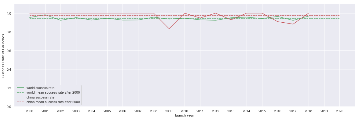
fig, ax = plt.subplots( figsize=(20,6.18) )

df_world_china.loc[2000:][ ['world success rate', 'world mean success rate after 2000' ] ].plot(ax=ax, color= 'g', style=['-', '--'] )
df_world_china.loc[2000:][ ['china success rate', 'china mean success rate after 2000' ] ].plot(ax=ax, color= 'r', style=['-', '--'] )
ax.set_xticks( df_world_china.loc[2000:].index.values )
ax.set_xticklabels( df_world_china.loc[2000:].index.values );
ax.set_ylabel('Success Rate of Launches')
ax.set_ylim([0,1.1])
fig.savefig('export/space-launch-success-rate-china-world-yearly.png')

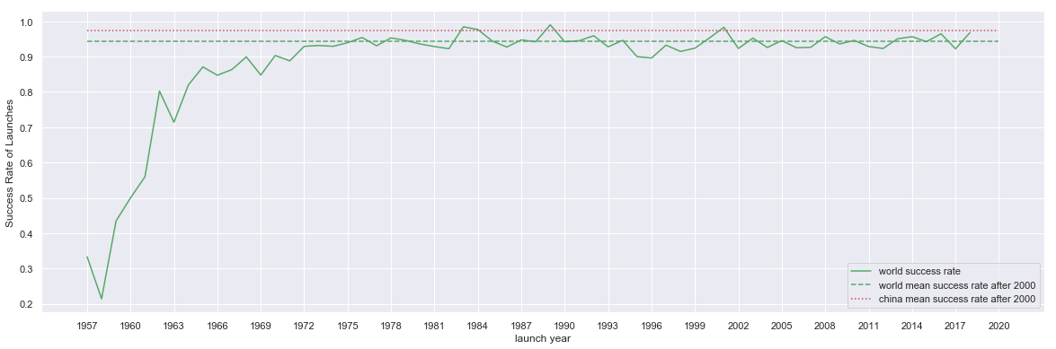
fig, ax = plt.subplots( figsize=(20,6.18) )

df_world_china[ ['world success rate', 'world mean success rate after 2000', 'china mean success rate after 2000' ] ].plot(ax=ax, color= ['g','g','r'], style=['-', '--', ':'] )
ax.set_xticks( launch_years[::3] )
ax.set_xticklabels( launch_years[::3] );
ax.set_ylabel('Success Rate of Launches')
fig.savefig('export/space-launch-success-rate-with-china-mean-yearly.png')

7.3. Air Transportation

df_air = pd.read_csv('data/air-transport-passengers-carried.csv')

df_air_t = df_air.transpose()

df_air_summary = df_air.describe()

df_air_summary

	1960	1961	1962	1963	1964	1965	1966	1967	1968	1969	...	2009	2010	2011	2012	2013	2014	2015	2016	2017	Unnamed: 62
count	0.0	0.0	0.0	0.0	0.0	0.0	0.0	0.0	0.0	0.0	...	1.820000e+02	2.050000e+02	2.050000e+02	2.050000e+02	2.040000e+02	2.040000e+02	2.000000e+02	2.010000e+02	1.990000e+02	0.0
mean	NaN	NaN	NaN	NaN	NaN	NaN	NaN	NaN	NaN	NaN	...	9.756383e+07	1.034285e+08	1.109374e+08	1.164027e+08	1.238505e+08	1.317110e+08	1.451395e+08	1.549384e+08	1.689135e+08	NaN
std	NaN	NaN	NaN	NaN	NaN	NaN	NaN	NaN	NaN	NaN	...	2.886695e+08	3.150289e+08	3.331397e+08	3.464099e+08	3.657630e+08	3.874896e+08	4.203152e+08	4.485057e+08	4.853347e+08	NaN
min	NaN	NaN	NaN	NaN	NaN	NaN	NaN	NaN	NaN	NaN	...	2.178400e+04	0.000000e+00	0.000000e+00	0.000000e+00	0.000000e+00	0.000000e+00	3.036000e+03	8.990000e+02	3.160000e+02	NaN
25%	NaN	NaN	NaN	NaN	NaN	NaN	NaN	NaN	NaN	NaN	...	7.521030e+05	5.705530e+05	5.441007e+05	6.501305e+05	6.244718e+05	6.073530e+05	8.418162e+05	6.670620e+05	7.839970e+05	NaN
50%	NaN	NaN	NaN	NaN	NaN	NaN	NaN	NaN	NaN	NaN	...	3.347920e+06	3.372283e+06	3.786453e+06	4.082595e+06	4.637628e+06	4.566060e+06	4.766130e+06	5.220218e+06	5.450671e+06	NaN
75%	NaN	NaN	NaN	NaN	NaN	NaN	NaN	NaN	NaN	NaN	...	3.165608e+07	3.621202e+07	3.898888e+07	3.996958e+07	4.353201e+07	4.492240e+07	5.041309e+07	5.381735e+07	5.836285e+07	NaN
max	NaN	NaN	NaN	NaN	NaN	NaN	NaN	NaN	NaN	NaN	...	2.249729e+09	2.628261e+09	2.786954e+09	2.894055e+09	3.048275e+09	3.227291e+09	3.466478e+09	3.705102e+09	3.978849e+09	NaN

8 rows × 59 columns

df_air_sum = pd.DataFrame( {
    'count': df_air_summary.loc['count'],
    'mean': df_air_summary.loc['mean'],
    'year': df_air_summary.columns
})

df_air_sum.dtypes

count    float64
mean     float64
year      object
dtype: object

df_air_sum['sum'] = df_air_sum.apply( lambda x: x['mean'] * x['count'], axis=1 )

df_air_sum

	count	mean	year	sum
1960	0.0	NaN	1960	NaN
1961	0.0	NaN	1961	NaN
1962	0.0	NaN	1962	NaN
1963	0.0	NaN	1963	NaN
1964	0.0	NaN	1964	NaN
1965	0.0	NaN	1965	NaN
1966	0.0	NaN	1966	NaN
1967	0.0	NaN	1967	NaN
1968	0.0	NaN	1968	NaN
1969	0.0	NaN	1969	NaN
1970	145.0	1.287005e+07	1970	1.866157e+09
1971	147.0	1.357727e+07	1971	1.995858e+09
1972	145.0	1.265414e+07	1972	1.834851e+09
1973	149.0	1.615547e+07	1973	2.407165e+09
1974	163.0	1.764458e+07	1974	2.876067e+09
1975	168.0	1.779737e+07	1975	2.989958e+09
1976	172.0	1.907453e+07	1976	3.280818e+09
1977	172.0	2.075610e+07	1977	3.570050e+09
1978	173.0	2.312858e+07	1978	4.001245e+09
1979	175.0	2.572554e+07	1979	4.501970e+09
1980	180.0	2.502693e+07	1980	4.504847e+09
1981	183.0	2.479053e+07	1981	4.536667e+09
1982	185.0	2.510708e+07	1982	4.644810e+09
1983	185.0	2.621469e+07	1983	4.849717e+09
1984	188.0	2.749760e+07	1984	5.169549e+09
1985	189.0	2.915406e+07	1985	5.510117e+09
1986	189.0	3.124599e+07	1986	5.905492e+09
1987	190.0	3.332837e+07	1987	6.332390e+09
1988	191.0	3.504809e+07	1988	6.694185e+09
1989	191.0	3.607536e+07	1989	6.890395e+09
1990	191.0	3.760631e+07	1990	7.182804e+09
1991	195.0	4.321195e+07	1991	8.426329e+09
1992	204.0	4.231283e+07	1992	8.631818e+09
1993	208.0	4.091522e+07	1993	8.510366e+09
1994	210.0	4.361480e+07	1994	9.159108e+09
1995	206.0	4.699636e+07	1995	9.681250e+09
1996	208.0	4.948879e+07	1996	1.029367e+10
1997	209.0	5.148545e+07	1997	1.076046e+10
1998	210.0	5.159658e+07	1998	1.083528e+10
1999	203.0	5.652634e+07	1999	1.147485e+10
2000	201.0	6.109103e+07	2000	1.227930e+10
2001	201.0	6.130171e+07	2001	1.232164e+10
2002	188.0	6.447087e+07	2002	1.212052e+10
2003	189.0	6.600647e+07	2003	1.247522e+10
2004	187.0	7.628911e+07	2004	1.426606e+10
2005	179.0	8.371204e+07	2005	1.498446e+10
2006	178.0	8.938296e+07	2006	1.591017e+10
2007	178.0	9.618326e+07	2007	1.712062e+10
2008	180.0	9.600924e+07	2008	1.728166e+10
2009	182.0	9.756383e+07	2009	1.775662e+10
2010	205.0	1.034285e+08	2010	2.120285e+10
2011	205.0	1.109374e+08	2011	2.274217e+10
2012	205.0	1.164027e+08	2012	2.386256e+10
2013	204.0	1.238505e+08	2013	2.526550e+10
2014	204.0	1.317110e+08	2014	2.686904e+10
2015	200.0	1.451395e+08	2015	2.902789e+10
2016	201.0	1.549384e+08	2016	3.114262e+10
2017	199.0	1.689135e+08	2017	3.361378e+10
Unnamed: 62	0.0	NaN	Unnamed: 62	NaN

df_air_sum.to_csv( 'data/air-transport-passengers-by-year.csv' )

7.4. Air Transportation and Death by Year

%%bash
ls data

air-transport-passengers-by-year.csv
air-transport-passengers-carried.csv
air-transportation-and-death-by-year.csv
space-exploration.csv

df_air_and_death = pd.read_csv('data/air-transportation-and-death-by-year.csv')
df_air_and_death.set_index('Year', inplace=True);

df_air_and_death.head()

	Deaths	Incidents	Total Passengers
Year
1970	2226	298	1866157152
1971	2228	271	1995858424
1972	3346	344	1834850740
1973	2814	333	2407165400
1974	2621	270	2876067000

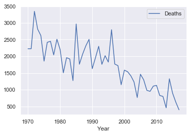
df_air_and_death[ ['Deaths'] ] .plot( )

<matplotlib.axes._subplots.AxesSubplot at 0x1a1a6d2cc0>

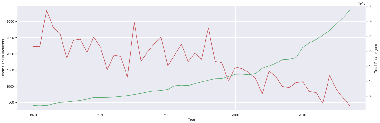
fig, ax1 = plt.subplots( figsize = (20,6.18) )

ax1.plot( df_air_and_death.index,  df_air_and_death['Deaths'], 'r' )
ax1.set_ylabel('Deaths Toll in Incidents')
ax1.set_xlabel('Year')

ax2 = ax1.twinx()

ax2.plot( df_air_and_death.index,  df_air_and_death['Total Passengers'], 'g' )
ax2.set_ylabel('Total Passengers')
ax2.grid(False)
#ax2.ticklabel_format(style='plain')

fig.savefig('export/air-transport-passengers-and-death-by-year.png')

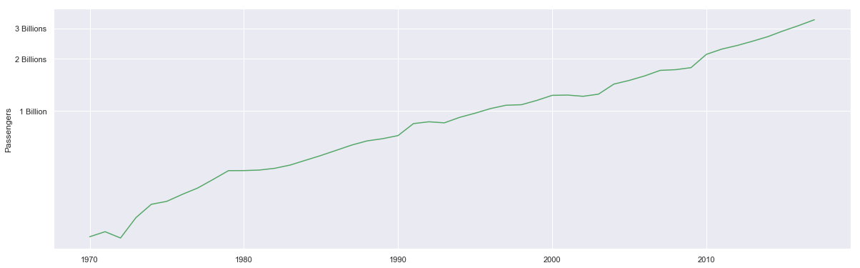
fig, ax = plt.subplots( figsize = (20,6.18) )


ax.semilogy( df_air_and_death.index,  df_air_and_death['Total Passengers'], 'g' )
ax.set_ylabel('Passengers')
ax.set_yticks( np.arange( 1*1e10, 4*1e10, 1e10 ) )
ax.set_yticklabels( ['1 Billion', '2 Billions', '3 Billions', '4 Billions'] )
#ax.grid(False)
#ax2.ticklabel_format(style='plain')

#fig.savefig('export/air-transport-passengers-by-year.png')

[Text(0,0,'1 Billion'), Text(0,0,'2 Billions'), Text(0,0,'3 Billions')]