Supply and Demand
Contents
72. Supply and Demand#
Some charts for supply and demand
import numpy as np
import matplotlib.pyplot as plt
from matplotlib import cm
from matplotlib.ticker import LinearLocator

import seaborn as sns;sns.set()
sns.set_style("darkgrid", {'axes.grid' : False})
72.1. Supply and Demand Demo Functions#
Demand function, only for illustration purpose.
class Demand():
    def __init__(self, **kwargs):
        self.params = kwargs

    def quantity_of_demand_wrt_price(self, p, **params):

        params__income = params.get(
            "income",
            self.params.get("income", 1)
        )
        if isinstance(p, (list, tuple,set)):
            max_p = max(p)
        else:
            max_p = max([p])
        params__intercept = params.get(
            "intercept",
            self.params.get("intercept", max_p)
        )

        return {
            "price": p,
            "quantity_of_demand": params__intercept-p + params__income
        }

    def __repr__(self):
        return f"Demand Function"


class Supply():
    def __init__(self, **kwargs):
        self.params = kwargs

    def quantity_of_supply_wrt_price(self, p, **params):

        params__stimulation = params.get(
            "stimulation",
            self.params.get("stimulation", 1)
        )

        return {
            "price": p,
            "quantity_of_supply": p - params__stimulation
        }

    def __repr__(self):
        return f"Supply Function"
dmd_params_1 = {"income": 1, "intercept": 11}
dmd_params_2 = {"income": 3, "intercept": 11}
dmd_1 = Demand(**dmd_params_1)
dmd_2 = Demand(**dmd_params_2)
dmd_p = np.linspace(1,11,101)
dmd_1_prices = dmd_1.quantity_of_demand_wrt_price(dmd_p)
dmd_2_prices = dmd_2.quantity_of_demand_wrt_price(dmd_p)
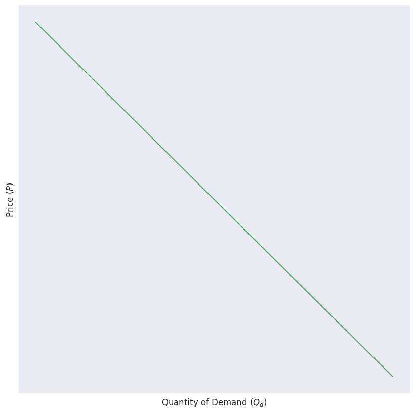
fig, ax = plt.subplots(figsize=(10, 10))

ax.plot(
    dmd_1_prices["quantity_of_demand"],
    dmd_1_prices["price"],
    "g-"
)

ax.set_xlabel(r"Quantity of Demand ($Q_d$)")
ax.set_ylabel(r"Price ($P$)")
ax.set_xticks([])
ax.set_yticks([])
[]
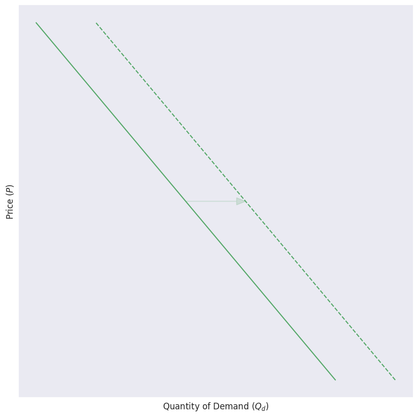
fig, ax = plt.subplots(figsize=(10, 10))

ax.plot(
    dmd_1_prices["quantity_of_demand"],
    dmd_1_prices["price"],
    "g-"
)

ax.plot(
    dmd_2_prices["quantity_of_demand"],
    dmd_2_prices["price"],
    "g--"
)

dmd_1_prices_qod_middle = dmd_1_prices["quantity_of_demand"][
    int(len(dmd_1_prices["quantity_of_demand"])/2)
]

dmd_1_prices_price_middle = dmd_1_prices["price"][
    int(len(dmd_1_prices["quantity_of_demand"])/2)
]

ax.arrow(
    dmd_1_prices_qod_middle, dmd_1_prices_price_middle,
    1.7, 0,
    fc="g", ec="g", head_width=0.2, alpha=0.2
)

ax.set_xlabel(r"Quantity of Demand ($Q_d$)")
ax.set_ylabel(r"Price ($P$)")
ax.set_xticks([])
ax.set_yticks([])
[]
sly_params_1 = {"stimulation": 1}
sly_params_2 = {"stimulation": 3}
sly_1 = Supply(**sly_params_1)
sly_2 = Supply(**sly_params_2)
sly_p = np.linspace(1,11,101)
sly_1_prices = sly_1.quantity_of_supply_wrt_price(sly_p)
sly_2_prices = sly_2.quantity_of_supply_wrt_price(sly_p)
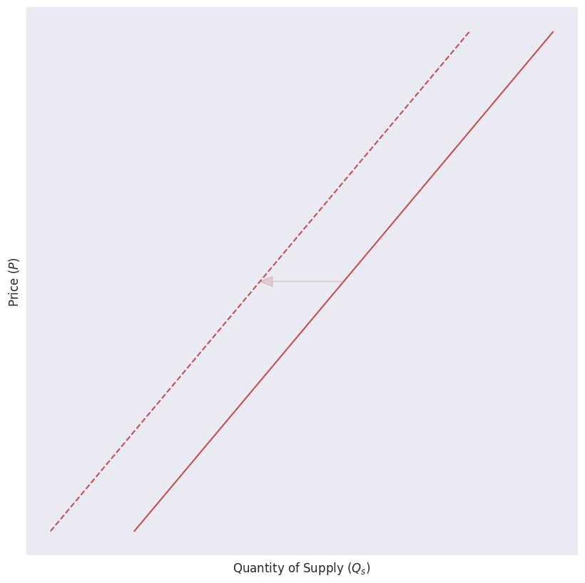
fig, ax = plt.subplots(figsize=(10, 10))

ax.plot(
    sly_1_prices["quantity_of_supply"],
    sly_1_prices["price"],
    "r-"
)

ax.plot(
    sly_2_prices["quantity_of_supply"],
    sly_2_prices["price"],
    "r--"
)

sly_1_prices_qos_middle = sly_1_prices["quantity_of_supply"][
    int(len(sly_1_prices["quantity_of_supply"])/2)
]

sly_1_prices_price_middle = sly_1_prices["price"][
    int(len(sly_1_prices["quantity_of_supply"])/2)
]

ax.arrow(
    sly_1_prices_qos_middle, sly_1_prices_price_middle,
    -1.7, 0,
    fc="r", ec="r", head_width=0.2, alpha=0.2
)

ax.set_xlabel(r"Quantity of Supply ($Q_s$)")
ax.set_ylabel(r"Price ($P$)")
ax.set_xticks([])
ax.set_yticks([])
[]
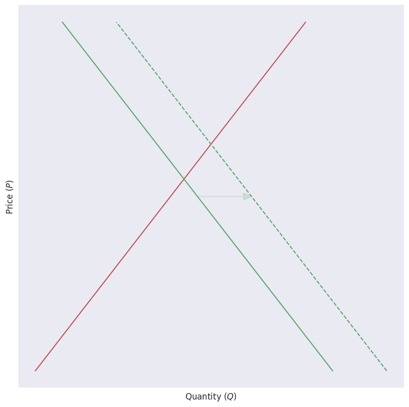
fig, ax = plt.subplots(figsize=(10, 10))

ax.plot(
    sly_1_prices["quantity_of_supply"],
    sly_1_prices["price"],
    "r-"
)


ax.plot(
    dmd_1_prices["quantity_of_demand"],
    dmd_1_prices["price"],
    "g-"
)

ax.plot(
    dmd_2_prices["quantity_of_demand"],
    dmd_2_prices["price"],
    "g--"
)

dmd_1_prices_qod_middle = dmd_1_prices["quantity_of_demand"][
    int(len(dmd_1_prices["quantity_of_demand"])/2)
]

dmd_1_prices_price_middle = dmd_1_prices["price"][
    int(len(dmd_1_prices["quantity_of_demand"])/2)
]

ax.arrow(
    dmd_1_prices_qod_middle, dmd_1_prices_price_middle,
    1.7, 0,
    fc="g", ec="g", head_width=0.2, alpha=0.2
)

ax.set_xlabel(r"Quantity ($Q$)")
ax.set_ylabel(r"Price ($P$)")
ax.set_xticks([])
ax.set_yticks([])
[]
incomes = np.linspace(0.1, 10.1, 10)
incomes
array([ 0.1       ,  1.21111111,  2.32222222,  3.43333333,  4.54444444,
        5.65555556,  6.76666667,  7.87777778,  8.98888889, 10.1       ])
dmd_p = np.linspace(1,11,101)
dmd_p
array([ 1. ,  1.1,  1.2,  1.3,  1.4,  1.5,  1.6,  1.7,  1.8,  1.9,  2. ,
        2.1,  2.2,  2.3,  2.4,  2.5,  2.6,  2.7,  2.8,  2.9,  3. ,  3.1,
        3.2,  3.3,  3.4,  3.5,  3.6,  3.7,  3.8,  3.9,  4. ,  4.1,  4.2,
        4.3,  4.4,  4.5,  4.6,  4.7,  4.8,  4.9,  5. ,  5.1,  5.2,  5.3,
        5.4,  5.5,  5.6,  5.7,  5.8,  5.9,  6. ,  6.1,  6.2,  6.3,  6.4,
        6.5,  6.6,  6.7,  6.8,  6.9,  7. ,  7.1,  7.2,  7.3,  7.4,  7.5,
        7.6,  7.7,  7.8,  7.9,  8. ,  8.1,  8.2,  8.3,  8.4,  8.5,  8.6,
        8.7,  8.8,  8.9,  9. ,  9.1,  9.2,  9.3,  9.4,  9.5,  9.6,  9.7,
        9.8,  9.9, 10. , 10.1, 10.2, 10.3, 10.4, 10.5, 10.6, 10.7, 10.8,
       10.9, 11. ])
prices_grid, incomes_grid = np.meshgrid(dmd_p, incomes)
prices_grid
array([[ 1. ,  1.1,  1.2, ..., 10.8, 10.9, 11. ],
       [ 1. ,  1.1,  1.2, ..., 10.8, 10.9, 11. ],
       [ 1. ,  1.1,  1.2, ..., 10.8, 10.9, 11. ],
       ...,
       [ 1. ,  1.1,  1.2, ..., 10.8, 10.9, 11. ],
       [ 1. ,  1.1,  1.2, ..., 10.8, 10.9, 11. ],
       [ 1. ,  1.1,  1.2, ..., 10.8, 10.9, 11. ]])
dmd_variable = Demand()

qod_variable = []
for i in range(len(incomes)):
    qod_i = []
    for j in range(len(dmd_p)):
        qod_i.append(
            dmd_variable.quantity_of_demand_wrt_price(prices_grid[i,j], income=incomes_grid[i,j], intercept=10)["quantity_of_demand"]
        )
    qod_variable.append(qod_i)

np.array(qod_variable).shape
(10, 101)
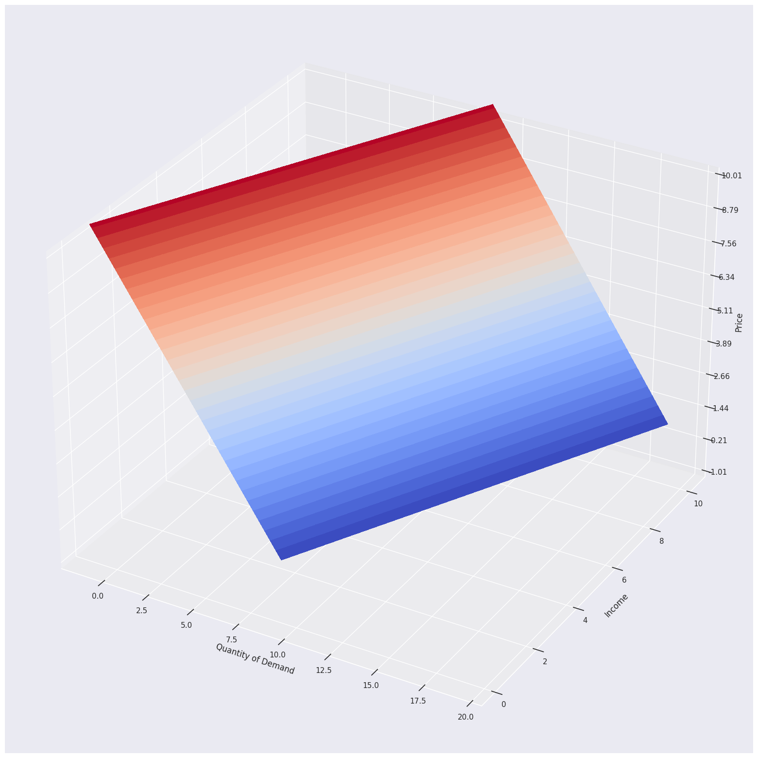
fig, ax = plt.subplots(subplot_kw={"projection": "3d"}, figsize=(20,20))

# Plot the surface.
surf = ax.plot_surface(qod_variable, incomes_grid, prices_grid, cmap=cm.coolwarm,
                       linewidth=0, antialiased=False)

# Customize the z axis.
ax.set_zlim(-1.01, 10.01)
ax.zaxis.set_major_locator(LinearLocator(10))
# A StrMethodFormatter is used automatically
ax.zaxis.set_major_formatter('{x:.02f}')
ax.set_xlabel("Quantity of Demand")
ax.set_ylabel("Income")
ax.set_zlabel("Price")

# Add a color bar which maps values to colors.
# fig.colorbar(surf, shrink=0.5, aspect=5)
Text(0.5, 0, 'Price')